Circuit Analysis#
For any circuit, we can use the following mathematical relations to determine what the voltage and current levels will be at a given time.
Ohm’s Law#
The three quantities voltage, current, and resistance are related through Ohm’s Law:
That is, the current through a resistor is linearly proportional to the applied voltage. We can show this linear relation in an IV-plot:
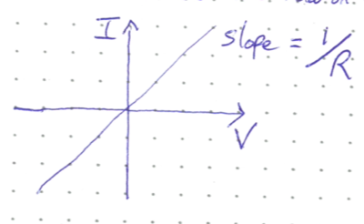
Alternatively, you can think about Ohm’s Law in terms of energy. Resistors dissipate energy, leading to a potential drop as current flows across the resistor. The amount of potential lost is equal to IR.
Kirchoff’s Current Law (KCL)#
The total current entering a junction is equal to the total current leaving the junction. For example, in the junction shown in the image below the arrows show the flow of current. In this case, KCL says that
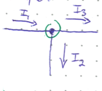
Notice the dot circled in green on the diagram. This is used to show that the wires are connected. As circuit diagrams get more complex throughout this course, remember that unless you see an explicit dot where wires cross, they are not connected.
Kirchoff’s Voltage Law (KVL)#
The sum of potential differences in any closed loop must equal zero. In the example image below, there are two closed loops labelled \(l_1\) and \(l_2\).
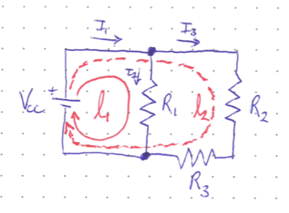
For loop one, the DC source starts at 0 V and pumps the voltage up to \(V_{CC}\) CC stands for common collector, a term that might make sense later on. For now though, \(V_{CC}\) is just an arbitrary voltage. The current goes around the loop, losing potential across \(R_1\). The amount of voltage lost is equal to \(I_2R_1\) from Ohm’s Law. The current then arrives back at its starting point. In mathematical terms, KVL states:
And for loop two, there are two resistors, and KVL thus gives:
If we know the value of \(V_{CC}\) and the three \(R\) values (which we typically do because we built the circuit), then combining the equations from KCL and KVL gives us a system of three equations ((2), (3), and (4)) and three unknowns (\(I_1\), \(I_2\), and \(I_3\)) which can be easily solved.
Concept Check:
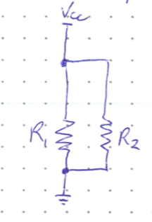
What is the voltage level at the top junction in the diagram above? What about the bottom junction?
Solution
Remember that our wires are considered perfect cunductors, and so the voltage is the same at every point on the wire. Since the top junction is connected to the high voltage terminal of the DC source, the voltage level is \(V_{CC}\). Similarly, The lower junction is connected to the lower voltage terminal and its voltage is thus 0 V.
Aside: Short Circuits
What would happen if \(R_1\) was removed from the circuit diagram, but the two points still connected?
In this case, the high voltage terminal is connected directly to the low voltage terminal with no resistance in between. Examining Ohm’s Law, we see that as \(R \to 0\), \(I \to \infty\). This is bad to put things mildly.
The massive amount of rapidly moving electrons in the current generate a ton of heat, and your circuit and sensitive components will quickly melt and be destroyed. Connecting high voltage directly to low is called a short circuit, and should be avoided. If you smell burning in lab, quickly unplug your circuit and don’t touch it until it has had time to cool.
Series and Parallel#
First some alternate notation for drawing circuit diagrams. In this course, we will use the ground symbol (three horizontal lines making a triangle) to simplify our diagrams. Anything connected to the ground terminal is at 0 V. Additionaly, current flows down from a high potential “rail” to ground, where it is implicitly assumed to loop back around to the high rail. Redrawing the KVL circuit thus looks like this:
The two resistors are said to be connected in parallel, because two parallel current streams flow through the resistors. This is opposed to being connected in series where the resistors are connected one after the other so there is only one current that flows through both resistors.
Often we talk about the equivalent resistance of a circuit. This is the resistance value we would need tou use if we replaced all of the resistors with only one resistor, but still get the same amount on current flowing down from the initial high rail.
For resistors connected in series, the equivalent resistance is simply a straight sum.
And for resistors connected in parallel like the diagram above, the equivalent resistance is
Example
Use Kirchoff’s Laws to prove the equivalent resistance relation for parallel resistors.
First we will draw in the currents and label them. \(I_0\) will flow directly from the high rail, and then split into \(I_1\) and \(I_2\) at the junction.
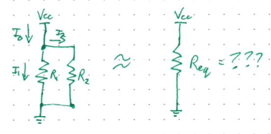
From Ohm’s Law we have
And from KCL we know
Rearranging the first three equations and plugging them into the last gives
The initial voltage cancels out and we are left with the expected relationship.